The Small Files Problem: Benchmarking S3, HDFS, and Greenplum Under Real Load

Not long ago, the Arenadata engineering blog published a benchmark examining how various distributed file systems behave under small-file workloads (~2 MB files). The headline finding: HDFS handles small files best, degrading by only 1.5×; MinIO-backed S3 fared worst at 8×; S3 API over Apache Ozone landed in between at 4×; and Greenplum was presented as the most capable system for small-file scenarios, including at exabyte scale. The authors also did extensive work tracing the "theoretical underpinnings of the unexpected results."

The S3/MinIO numbers didn't sit right with our team. We suspected the results might stem from:

• Limited hands-on experience operating SQL-over-S3 stacks and S3 in general;

• Differences in distribution builds and default configurations;

• Lack of experience running production MinIO clusters — specifically in high-throughput environments with 200+ TB of compressed columnar Iceberg/Parquet data, exactly the scenarios where the small-file problem surfaces fastest.

We're grateful to our colleagues for the inspiration. Let's run the experiment ourselves.

Environment

The test environment was provisioned on cloud IaaS infrastructure.

MinIO node configuration:

Nodes	4
vCores	8
RAM (GB)	32
Storage	4 network SSD drives × 1024 GB each per node (16 network drives total across the cluster)

For the SQL engine we used Impala 4.5_2025.04 — part of the Alphyn Lakehouse 2025.04 release.

Impala Kubernetes node configuration:

Nodes	4
vCores	32
RAM (GB)	252

Local data caching on the Impala worker nodes was disabled entirely so that all reads during the test went directly to S3.

The cluster was intentionally skewed toward compute resources so that storage would become the bottleneck if problems arose. Both MinIO and the SQL engine were tuned for maximum performance — at the cloud infrastructure level, the OS level, and through individual component settings. Extensive production experience with systems like this has given us a solid foundation of tuning know-how.

Experiment Design

The benchmark followed the TPC-DS methodology. Rather than a single sequential run of 99 SQL queries, we ran 4 simultaneous TPC-DS streams — 396 queries in total — all executing concurrently and strictly complying with the methodology's requirements for concurrent execution. The goal was to create the most hostile possible workload for the object store: we wanted to see "bad MinIO" choke on the torrent of list and small-file read requests from the engine, and to put the original article's "theoretical deep-dive" section to a proper test.

Arenadata considered 2.3 MB a reasonably small file size, representative of Change Data Capture patterns — especially on HDFS. We decided to start from the absolute worst case and climb up from there. Data was prepared with Spark in Parquet format across 14 schemas, each targeting a specific file size ranging from 256 KB to 128 MB.

Experiment #	File size (MB)	File count in S3
1	128	248
2	96	322
3	64	463
4	48	612
5	32	956
6	24	1,339
7	16	1,878
8	12	3,338
9	8	7,037
10	4	11,733
11	2	28,107
12	1	46,836
13	0.5	102,178
14	0.25	140,102

At the worst-case point, our dataset contained 10× more files than the Arenadata test — 140,000 vs. 14,000.

We deliberately covered the full spectrum between the smallest and largest file sizes to capture the degradation curve, not just the endpoints.

Results

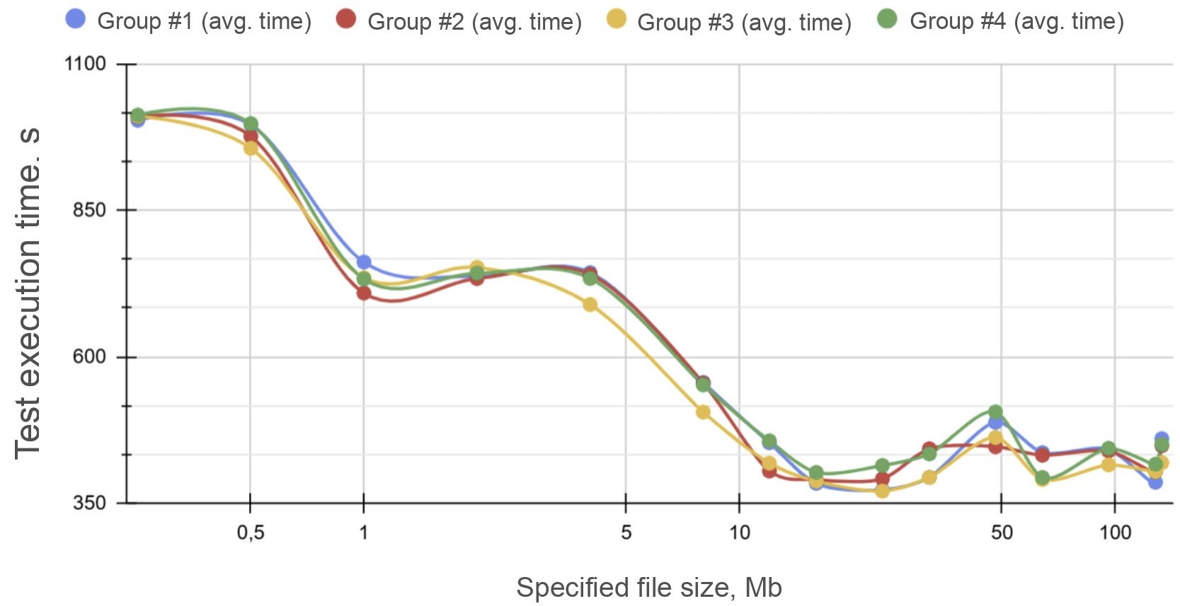
The charts below show completion times for each of the 4 independent TPC-DS streams running simultaneously:

• Y-axis: elapsed time in seconds, stepped at 125 s;

• X-axis (log scale): file size in MB.

For cleaner analysis, the chart below shows overall test completion time — defined as the slowest stream in each group.

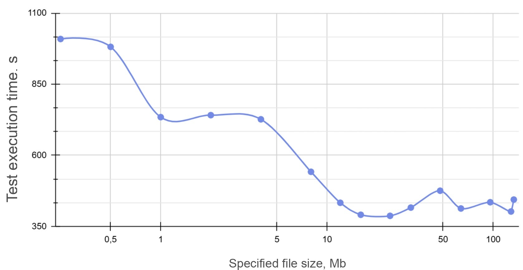
Chart: TPC-DS 4-stream total time vs. file size:

• Y-axis: elapsed time in seconds, stepped at 125 s;

• X-axis (log scale): file size in MB.

The same results in tabular form:

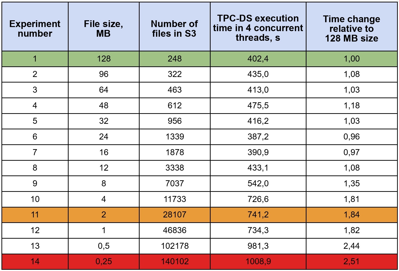
Absolute times are not the interesting metric here. What matters is how each scenario compares to our baseline of 128 MB files.

Key Findings

• At the 2 MB reference point — the result is 1.8× slower. (Recall the Arenadata results with 10× fewer files: HDFS 1.5×, S3 API Ozone 4×, MinIO 8×.)

• In our experiment, significant degradation (beyond 1.8×) only appeared below 4 MB file sizes.

• Files in the 10–12 MB range can still be considered operationally acceptable, but degradation accelerates below that threshold:

  • Our production best-practice for peak performance: the cluster-wide average file size (total volume ÷ total file count) should not fall below 30–40 MB.

• Maximum observed degradation was 2.5× relative to the 128 MB baseline, recorded at 256 KB.

• Even though our object store was hit with several times more requests than in the reference benchmark, our maximum degradation — 2.5× at 256 KB and 1.8× at 2 MB — is nowhere near the 10× (1000%+) reported by the original authors. And this was under 40× higher I/O load from the SQL engine than their test generated.

Rather than backing these results up with internet citations and PDF-style analytical memos, we'll simply invite you to bring our team on-site for a live test so you can see the results firsthand.

Does the Small Files Problem Actually Exist?

Absolutely — it does. In Lakehouse and Data Lake architectures, proactively managing small files is essential: you need to monitor average file size and compact before degradation sets in. The problem is most acute in real-time ingestion scenarios, where compaction and table maintenance must be configured before the data stream is connected.

Left unchecked, the issue doesn't just hurt performance — for Iceberg tables (now mainstream) it can make them operationally unmanageable. At that point you may need a disproportionate amount of cluster resources just to run a compaction. Read queries slow dramatically at the SQL-compute layer because the engine has to read 100× more files and Iceberg metadata.

Alphyn Lakehouse includes a built-in managed Iceberg maintenance service with a graphical interface — fully integrated into the platform — so users don't have to build their own compaction tooling from scratch.

What About HDFS?

In practice, the HDFS NameNode tops out at 200–300 M files regardless of their size. The absolute theoretical ceiling is 2³¹ (2 billion) inodes in the fsimage, but that number is never reached in real deployments.

Why? Several reasons stack up:

• JVM heap memory on the NameNode and GC pressure from large heaps. At 150 M objects, heap footprint runs around 100 GB.

• HDFS snapshots are widely used in large production clusters — at minimum for replication and change isolation without open table formats. With 5 snapshots per object and just 5% object churn per snapshot (conservative estimates — in practice on a 5 PB HDFS cluster I've seen snapshotting consume up to 20% of total volume at 3 snapshots per object), heap grows by ~1.3×: ~130 GB for 150 M objects, ~260 GB for 300 M objects.

• The calculations above assume columnar files like Parquet or ORC. Add Iceberg to the picture and the situation changes materially. Iceberg introduces a large number of metadata files — roughly as many as data files — plus delete files from accumulated changes, fragmented data files, and versioning overhead. The practical result: the "useful" quota (actual data files in the current Iceberg snapshot) drops to roughly 30–50 M objects per NameNode, with all remaining capacity consumed by Iceberg housekeeping. And don't overlook availability: NameNode startup in production typically takes ~30 minutes.

How is the small files problem handled in HDFS? First and foremost, by monitoring average file size and merging small files into larger ones. For Iceberg — as with S3 — regular compaction of data files and manifest files helps. When the file count still exceeds the practical limit even after regular maintenance, teams resort to HDFS Federation, but that dramatically increases operational complexity because:

• Each NameNode requires its own HA setup;

• Namespaces are isolated: cross-namespace moves are not possible — only copies;

• Load balancing across NameNodes becomes manual: there is no automatic distribution, data placement must be planned by hand, and DataNodes can become overloaded by a single namespace;

• Operational overhead multiplies: backup/restore/replication, HA configuration, version upgrades, quota management (per namespace), resource governance, and the skill requirements for administrators all grow substantially.

These are exactly the pain points that drove large HDFS Federation deployments to migrate to native S3 solutions (Ceph, MinIO, public cloud S3) — and the same pain that motivated the creation of Apache Ozone in the first place.

What About Greenplum?

First, a few well-known facts about how PostgreSQL and Greenplum are structured internally:

1. In PostgreSQL, every partition of every table has its own set of data files:

   1. Data files with page-level internal organization, split at 1 GB boundaries (each additional gigabyte is a new file);

   2. Auxiliary files: free space map (FSM), visibility map (VM), _init (for unlogged tables);

   3. Index files (if indexes exist).

2. Greenplum is composed of segments. A single physical host runs 4 to 8 segments; each segment is a PostgreSQL instance, plus one active shared master and its standby.

3. The primary table type for analytics and DWH in Greenplum is Append-Only Column-Oriented (AOCO): per segment, per partition, per column — a separate data file, following the same split logic as item 1. In addition to visible columns there are 33 technical columns per AOCO table, each with its own file per partition.

4. The second key table type is AOT Row — Append-Only Row-Oriented, which uses compression but stores data row-wise. It's significantly less optimal for HTAP/OLAP workloads on large clusters (lower compression ratio, no columnar reads). Its file structure is closer to standard PostgreSQL: one data file per 1 GB per partition.

5. All large tables must be distributed close to uniformly across all segments (which are the units of parallelism). Each segment therefore holds a slice of every partition, with all its associated files, for parallel processing — storage and compute are tightly coupled in a symmetric MPP design.

6. The pg_catalog is replicated to every segment.

In the discussion that follows, "partition count" (or more precisely, "pg_catalog object count") refers to the sum of all non-partitioned tables plus the sum of all partitions across all partitioned tables in the entire cluster.

A Real Experiment: pg_catalog Degradation in Practice

1. Testbed configuration:

   1. Dedicated on-premises hardware, 4 segment hosts with 64 CPU cores, 1 TB RAM, 8 segments per host;

   2. Storage subsystem: 2 RAID-10 arrays of 4× Enterprise NVMe PCIe Gen4 ×4 drives each (8 drives total per host);

   3. 100 GbE local network with an additional 100 GbE bonding for redundancy.

(!) All figures from this experiment represent best-case performance, thanks to NVMe storage and 100 GbE network bandwidth.

2. We created 331 AOCO tables, each with 100 columns (133 including technical columns). Total across all tables: 5.4 M partitions, 32 M small files per segment (!). At this point the tables contained zero rows — column-level files don't exist until the first INSERT. Once any row lands in a partition, that segment gains +100 files for that partition. With all partitions populated, that's at minimum 100× the partition count in per-segment files — roughly 15× for this particular case. The appearance of per-column files doesn't affect catalog behavior directly, but it dramatically changes SELECT/DML performance and the host filesystem — though that's the next stage of testing. We're focusing on catalog effects here, because unfortunately the cluster grinds to a halt at this point already.

3. The system catalog occupied 12 TB before VACUUM (see chart below) and 9 TB after — largely because it is replicated across all segments. The data files with zero actual rows consumed 11 TB — real big data on a literally empty dataset.

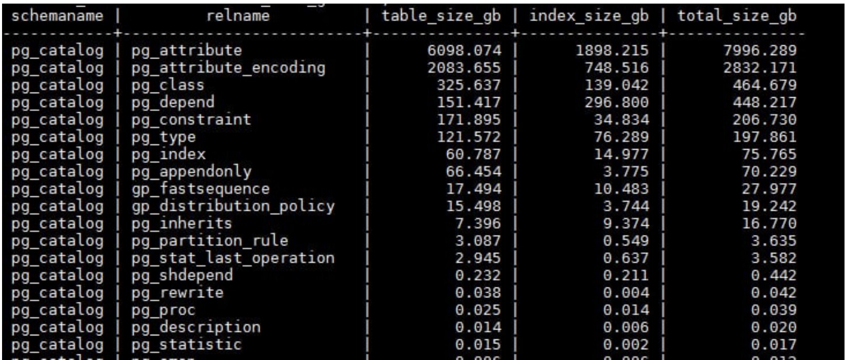
4. Measurements and findings with 0 rows in AOCO tables:

   1. At 400 K partitions (chosen as the most representative point for large clusters), catalog queries already degrade to 5 seconds;

   2. At 5.4 M partitions — degradation exceeds one minute (75 seconds; 55 seconds after VACUUM FULL on the system catalog);

   3. Degradation is linear: each additional 10 K empty partitions adds ~100 ms;

   4. At 5.4 M partitions: a non-concurrent DDL in a single session (CREATE of a new empty table with 1,000 partitions) takes 10 seconds; DROP of an empty table takes 10 minutes;

   5. Concurrent DML/DDL across 80–100 sessions against the catalog at 400 K partitions brings the entire cluster to a complete halt.

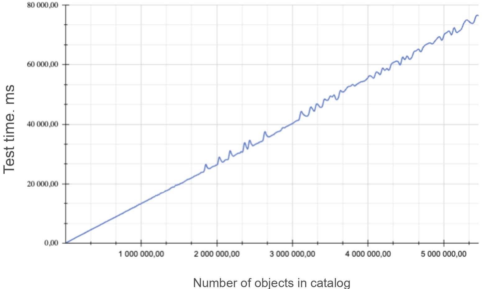
5. AOT Row fares better: 1 M AOT Row partitions with 500 concurrent queries on the NVMe testbed described above, with proper tuning, is the threshold at which the cluster still doesn't degrade on pg_catalog access.

In production workloads, concurrent session count matters enormously — and the query optimizer itself hits the catalog on every query.

The practical architectural limits of Greenplum are therefore:

• AOCO: ~300 K partitions per cluster on a well-provisioned NVMe-based physical cluster, with ~100 concurrent sessions at minimal load — a hard ceiling independent of hardware for a single GP cluster;

• AOT Row: ~1 M partitions and ~500 sessions for NVMe storage with sufficient RAM.

The resulting compounding slowdown of SELECT/DML/DDL operations, cluster stalls during catalog and data-file VACUUM, and overall degradation of maintenance operations (backup, restore, replication) is known as GP catalog bloat.

As much as one might wish otherwise, Greenplum cannot handle large numbers of small files due to its architecture — it gets stuck on the very first step: listing objects in pg_catalog.

Conclusions

On one hand, we ran an extreme experiment with 5.4 M Greenplum partitions — a number that borders on fiction in practice. But we're not the ones claiming that Greenplum scales to petabytes of compressed data under meaningful concurrent load.

On the other hand, large real-world GP clusters running a few hundred terabytes typically do accumulate 100–400 K AOCO partitions — which, as we've seen, is already close to the technology's practical ceiling for a single cluster.

Credit for the Greenplum experiment and analysis goes to Mark Lebedev and his team. Mark recently published an excellent deep-dive comparing Greenplum 6, Greenplum 7, and Cloudberry — well worth reading.

The findings from all three systems point in the same direction: S3-based object storage with a well-tuned MinIO cluster is far more resilient to the small files problem than commonly assumed, while both HDFS and Greenplum carry hard architectural ceilings that become real constraints at scale. Managing file sizes proactively — and using built-in compaction tooling — remains the right answer regardless of the underlying storage system.

---

See it on your own data

If you're weighing how this would handle your workloads, we'd be glad to walk you through Alphyn Lakehouse on a real scenario. Book a sovereign-lakehouse walkthrough →

---