Terabytes of Data from Teradata to Trino: An Efficient Transfer Method

The Lakehouse architectural principle assumes you operate on all data loaded into the system. But sometimes you need to perform ad hoc analysis outside its perimeter — because the data you need isn't available in the Lakehouse platform for one reason or another. This is where federated access comes to the rescue. The standard engine for this task is Trino. It can extract data from external databases and, in some cases, even push down certain computations to the source system. The key requirement is having a suitable connector for the target database that can work with it efficiently.

Recently, a new Trino Teradata Connector was added to Alphyn Lakehouse. It allows users to pull the necessary data slices from Teradata as part of ad hoc queries and solves the problem of efficient data transfer: you can move terabytes across multiple threads without significantly increasing the load on the source.

In this article, we will cover:

• How to organize efficient multi-threaded work with Teradata:

  • Where mistakes are commonly made;

  • What a correct solution looks like;

• What capabilities the Alphyn Lakehouse Trino Teradata Connector provides:

  • Multi-threaded extraction;

  • Push-down optimizations.

A note before we begin

First, it is worth noting that we do not recommend using the Alphyn Lakehouse Trino Teradata Connector specifically for data migration into a Lakehouse platform or for regular batch loading. We have a specialized tool for efficient batch data transfer — Alphyn Alphyn Data Replicator — which, when working with Teradata, uses (at the user's or administrator's choice) either the Native Object Storage (NOS) mechanism or Teradata Parallel Transporter (TPT). The need for Trino-based access among our customers typically arises in federated use cases such as data reconciliation, data quality validation, source system data profiling, and so on.

Efficient Client Access to Teradata

A Brief Look at Teradata Architecture

A deep dive into the Teradata DBMS is not the goal of this article, but to make the remaining technical details clear and help everything come together by the end, we will briefly touch on the key architectural aspects. We expect more readers may be familiar with Greenplum, so we will also draw parallels with it.

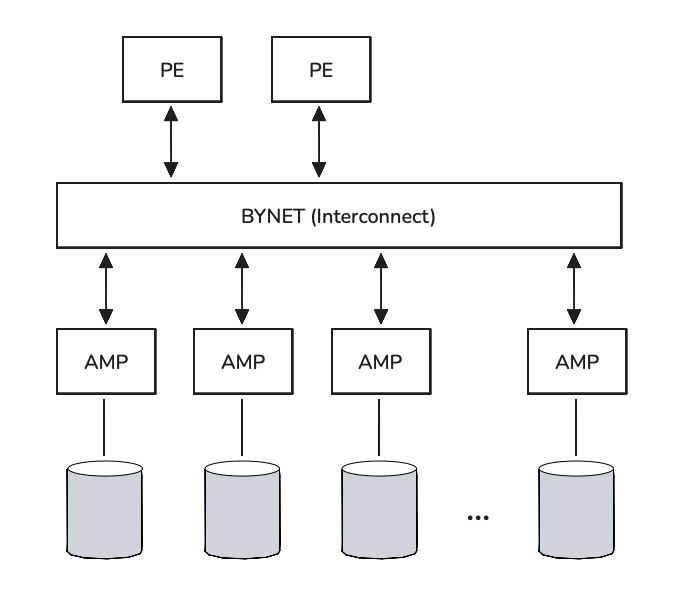
Teradata is a shared-nothing MPP DBMS: each worker node has its own dedicated compute resources (CPU, RAM, Disk). Worker nodes are called AMPs (Access Module Processors; the full name is rarely used), and table rows are distributed across AMPs for storage and processing. AMPs are connected via the BYNET interconnect network. Users connect and send queries to Parsing Engine (PE) components — this is where query parsing, plan construction, task distribution to AMPs, execution control, and result assembly and delivery to the client all happen.

Teradata was designed a long time ago, when memory was far scarcer and far more expensive (though, publishing this article in early 2026, it is hard to talk about cheap memory either). The DBMS was therefore designed from the start to actively use the disk subsystem for intermediate computations and prepared result sets — this design persists today. In query plans, you will frequently see the DBMS writing to Spool — that is exactly this mechanism.

For those familiar with Greenplum, here is a quick analogy:

• Master Server → Parsing Engine (PE), of which there can be several; each PE can handle around 100+ sessions;

• Segment → AMP. Typically, several Segment Servers run on a single, fairly powerful physical Segment Host, but an equivalently powerful Teradata Node always has more AMPs, so the total AMP count in Teradata is usually higher — numbering in the hundreds or thousands. However, each individual AMP has fewer resources at its disposal and stores/processes less data than a single Segment;

• Distributed Key → Primary Index. Data is distributed across worker nodes by hashing the fields in the distribution key. The goal is typically to achieve an even distribution of data across worker nodes for large tables (smaller tables usually use a different storage strategy). There are quite a few differences in the implementation details of data distribution and storage, but we will not go deeper into them here — let's stay focused on the main goals of this article;

• Spill → Spool. Unlike Greenplum, which tries to keep computations in RAM until it runs out, Teradata will write to Spool right away.

Where Mistakes Are Commonly Made

Over the years, we have encountered numerous solutions for extracting data from Teradata and loading it into Hadoop or a Lakehouse, and many of them shared the same efficiency problems. And not just because some extracted hundreds of GBs in a single thread. The more critical issue is when extraction in N threads creates N times the load on the source system.

For parallel extraction in such cases, multiple queries were constructed, each responsible for processing its own portion of rows (there are two common variants):

SELECT ... FROM table WHERE hashbucket(hashrow(key_field)) MOD 4 = 0;
SELECT ... FROM table WHERE hashbucket(hashrow(key_field)) MOD 4 = 1;
SELECT ... FROM table WHERE hashbucket(hashrow(key_field)) MOD 4 = 2;
SELECT ... FROM table WHERE hashbucket(hashrow(key_field)) MOD 4 = 3;

SELECT ... FROM table WHERE hashamp(hashbucket(hashrow(key_field))) MOD 4 = 0;
SELECT ... FROM table WHERE hashamp(hashbucket(hashrow(key_field))) MOD 4 = 1;
SELECT ... FROM table WHERE hashamp(hashbucket(hashrow(key_field))) MOD 4 = 2;
SELECT ... FROM table WHERE hashamp(hashbucket(hashrow(key_field))) MOD 4 = 3;

Each of these queries will indeed return its own non-overlapping portion of rows (we will set aside the case of concurrent modifications for simplicity). But what did the DBMS have to do to produce these results? What work was actually performed?

To process each query, every AMP scans all of its rows and checks which ones satisfy the condition hash(key_field) MOD 4 = X. Matching rows are written to Spool by each AMP. Then each AMP returns those rows from Spool to the client. In other words, during a single such query we scan the entire table, spend additional CPU computing predicates for every row, and only after that does any resource savings begin.

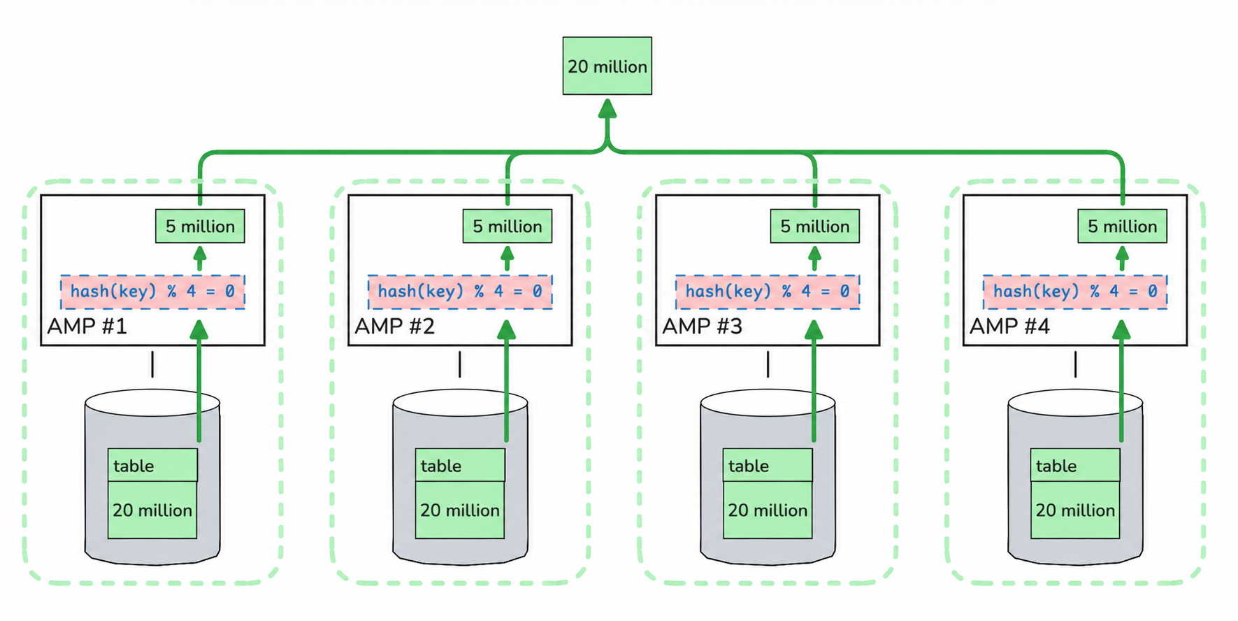
But we are not running just one such query — we are running N of them. This means extraction in N threads results in N full table scans: as we increase the number of threads, we linearly increase the load on the source system. Want to extract a 10 TB table from Teradata into a Lakehouse, but a single thread is too slow? Use 10 threads and force 10 times more work — instead of scanning 10 TB through the I/O subsystem, we push 100 TB through it plus burn a huge amount of CPU computing predicates.

In summary, this method scales very poorly. Extraction in N threads produces:

• N-fold increase in I/O operations in Teradata;

• N-fold increase in CPU load in Teradata;

• Minimal reduction in extraction time. Data preparation time on the Teradata side does not decrease; the only gain comes from reducing the data volume per thread on the receiving side.

What Efficient Extraction Requires

Let's examine what we have at the point when we want to extract data from Teradata and what we know about it:

• The table data is already distributed across hundreds of AMPs (and in large installations, across several thousand);

• Each AMP holds a roughly equal portion of data;

• Since there are enough portions (hundreds to thousands), there is no need to split them further at extraction time — on the contrary, data from multiple AMPs can be extracted within a single thread (connection/session).

You can draw a parallel with table partitioning, which is widely used across various DBMSs, including Teradata. Partitioning lays data out into separate portions (partitions) so you can read just one specific partition rather than scanning everything. In our case, we want to read the portion on a specific AMP within a single extraction thread.

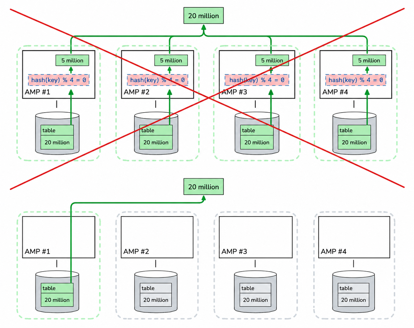
Teradata provides exactly this mechanism — you can retrieve data from a specific AMP by specifying its ordinal number. You can also specify multiple AMPs at once, which is very convenient for designing different workloads for different scenarios.

Knowing the number of AMPs, we can distribute the extraction task across N threads. For example, with 10 processes running on the Lakehouse side and a Teradata cluster with 1000 AMPs, the distribution would look like this:

• AMPs [1, 2, 3, … 100] → worker 1

• AMPs [101, 102, 103, … 200] → worker 2

• ...

• AMPs [901, 902, 903, … 1000] → worker 10

With this approach, each AMP reads its portion of data exactly once, regardless of the number of threads. This eliminates the scaling problems described earlier:

• N-fold increase in I/O operations in Teradata → The number of I/O operations is constant for a given table, regardless of thread count;

• N-fold increase in CPU load in Teradata → CPU load on AMPs is constant for a given table, regardless of thread count;

• Minimal reduction in extraction time → Extraction time decreases linearly, provided all queries actually run in parallel.

To close out this section, a note about computation Skew. In the extreme case, a single query reads data from just one AMP, meaning all computation happens on a single AMP — this corresponds to 100% Skew. Normally, such heavy skew is something to avoid, so system administrators sometimes raise concerns about these queries. The explanation is straightforward: if you sum up all the queries — each of which pulled its portion of data from one AMP (and therefore showed 100% Skew in its metrics) — the aggregate across all queries will show 0–1–2% Skew, which corresponds to the skew of the source table itself.

Trino Teradata Connector in Alphyn Lakehouse

The proper Teradata Connector is now included in the Alphyn Lakehouse distribution. No additional installation steps are required — you can go straight to configuring a catalog that will allow Trino to connect to one of your Teradata clusters:

CREATE CATALOG teradata_cluster USING teradata
WITH (
  "connection-url" = 'jdbc:teradata://hostname/DATABASE=mydb,DBS_PORT=1025',
  -- Using credential passthrough
  "user-credential-name" = 'td_user',
  "password-credential-name" = 'td_password'

  -- Alternative: specify a shared technical account
  -- "connection-user" = 'user',
  -- "connection-password" = 'password'
);

Immediately after this, you can send queries from Trino that interact with Teradata:

SELECT * FROM teradata_cluster.db_name.table_name WHERE ...
;

SELECT ...
FROM lakehouse_db.lakehouse_table
LEFT JOIN teradata_cluster.db_name.table_name ON ...
WHERE ...
;

During execution of these queries, Trino reads data from Teradata. By default, reads happen in a single thread, but this is easy to change:

SET SESSION teradata_cluster.max_scan_parallelism = 4;

The connector automatically determines the number of AMPs in Teradata and distributes the extraction across Trino Workers:

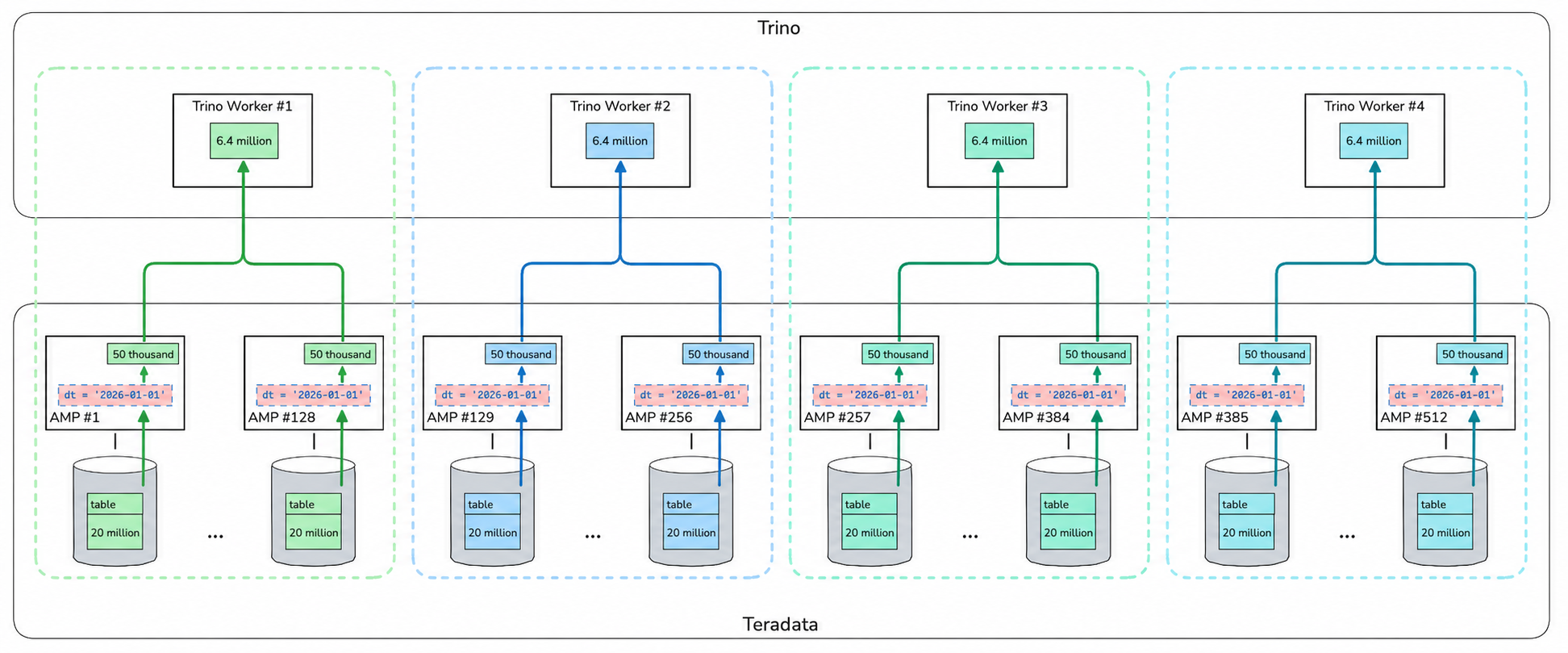
Each AMP scans its data exactly once regardless of the number of extraction threads. If max_scan_parallelism is set higher than the number of AMPs, the thread count will equal the AMP count — no more. In that case, each thread extracts from exactly one AMP. In practice, 4–8–16 threads are sufficient for fast extraction depending on table size — you are unlikely to ever hit this upper limit.

The diagram above shows an additional filtering step — in this example, Trino only needs data for a single day. It makes sense to filter out unnecessary data on the source side and avoid transferring it at all — Trino can push down certain expressions to the source to optimize transfer volumes.

Supported Push-Down Optimizations

WHERE Predicate Push-Down

To filter the result set on the source side, Trino can push down certain operators and functions (and their combinations via AND/OR). The Teradata Connector currently supports:

• Comparison operators: =, <>, <, <=, >, >=;

• Arithmetic operations on integer types: +, -, *, /, MOD;

• Unary minus for integer types;

• The LIKE operator (with optional ESCAPE);

• NULL checks: IS NULL, IS NOT NULL;

• Logical negation: NOT;

• The NULLIF function;

For example:

SELECT dt, client_id, phone_number
FROM teradata_cluster.db_name.table_name
WHERE dt = '2026-01-01' AND phone_number IS NOT NULL;

Aggregation Function Push-Down

Aggregation typically reduces the result set size, so push-down can also reduce the volume of data transferred. The result may be substantially smaller than the full dataset, which can significantly improve execution time — especially when the final output is orders of magnitude smaller (10x, 100x, 1000x).

However, since the original user query in Trino can contain any aggregation that Trino supports, it is important that the target DBMS has equivalent functions and that the connector knows how to translate them. The Teradata Connector currently supports a standard set: COUNT/COUNT(DISTINCT), SUM, MIN, MAX, AVG, as well as the less commonly used STDDEV_SAMP, STDDEV_POP, VARIANCE, and VAR_POP. The following query, for example, can be pushed down to Teradata for execution:

SELECT report_dt, COUNT(*), AVG(salary)
FROM teradata_cluster.db_name.table_name
GROUP BY report_dt;

An important note: if even one aggregation function in a query is not supported for push-down, all aggregations in that query will be executed in Trino. If the calculation requires pulling detailed data anyway, it is more efficient to make a single computation pass in Trino than to make two passes (one in Trino and one in the source DBMS).

If aggregation push-down is not needed, it can be disabled:

SET SESSION teradata_cluster.aggregation_pushdown_enabled = false;

JOIN Push-Down

An important disclaimer upfront: join push-down only works for objects within the same catalog. If a query references objects from different catalogs, Trino will load data from each object locally and perform the join itself. No magic here — at least not yet.

It is also important that join conditions do not contain any Trino-specific functions that have no equivalent in Teradata.

Beyond those caveats, this is another good way to reduce the result set size before transferring data to Trino — especially when the data volume decreases significantly.

However, if the join is expected to increase the number of rows, it is better not to push it down. You can pull the emergency brake like this:

SET SESSION teradata_cluster.join_pushdown_enabled = false;

Limitations of Push-Down Computations in Teradata

Earlier we discussed fast extraction of the resulting dataset from Teradata in N threads. For this, each thread must pick up ready-made data from one or more AMPs. Adding a filter condition (WHERE predicate) on top of this is straightforward — it can be applied independently on each AMP.

But when it comes to joins or aggregations, the problem changes fundamentally. The system can no longer simply return stored data with simple scalar computations applied — it must perform much more complex work, which may include:

• Redistribution of one or more tables across AMPs;

• Duplication of a table to all AMPs;

• Additional sorting of rows on each AMP for one or more tables;

• Building a hash table.

These computations cannot be confined to a single AMP — correct operation requires data from other AMPs. Therefore, each extraction thread will engage not just one or a few specified AMPs, but all of them. We covered the problems associated with this at the beginning of the article.

What options are available in this case?

1. "Push-Down Priority." Push down the join/aggregation + extract in a single thread;

2. "Multi-Threaded Extraction." Disable push-down and extract in parallel;

3. "Materialization." Run a CREATE TABLE AS SELECT with the required join/aggregation in Teradata, then extract multi-threaded.

The right approach depends on many specific conditions, but here are general recommendations for several scenarios:

• If the final result set is small — go with "Push-Down Priority";

• If the result set is significantly reduced by the operation, you can typically use "Push-Down Priority" or "Materialization" (when there is available space in the Teradata sandbox);

• If the result set stays roughly the same size after the join/aggregation — go with "Multi-Threaded Extraction", since you need to transfer the same volume regardless.

Conclusion

To wrap up, here are the key ideas and takeaways:

• For efficient multi-threaded data extraction from Teradata, each thread should work with its own subset of AMPs. Each AMP should be engaged exactly once, regardless of the number of threads;

• In some cases, it may be more efficient to perform computations on the source side to reduce the result set size. Trino can push down certain computations, but the connector must support them as well;

• When pushing down computations, it is important to understand how they will be executed on the source — some should not be combined with multi-threaded extraction. But this can still be the better choice, especially when the resulting dataset is substantially smaller.

---

See it on your own data

If you're weighing how this would handle your workloads, we'd be glad to walk you through Alphyn Lakehouse on a real scenario. Book a sovereign-lakehouse walkthrough →

---